A. Uncertainty Quantification#
A.1. Introduction#
As defined in Chapter 1, uncertainty quantification (UQ) refers to the formal focus on the full specification of likelihoods as well as distributional forms necessary to infer the joint probabilistic response across all modeled factors of interest [8]. This is in contrast to UC (the primary focus of the main document of this book), which is instead aimed at identifying which modeling choices yield the most consequential changes or outcomes and exploring alternative hypotheses related to the form and function of modeled systems [9, 10].
UQ is important for quantifying the relative merits of hypotheses for at least three main reasons. First, identifying model parameters that are consistent with observations is an important part of model development. Due to several effects, including correlations between parameters, simplified or incomplete model structures (relative to the full real-world dynamics), and uncertainty in the observations, many different combinations of parameter values can be consistent with the model structure and the observations to varying extents. Accounting for this uncertainty is conceptually preferable to selecting a single “best fit” parameter vector, particularly as consistency with historical or present observations does not necessarily guarantee skillful future projections.
The act of quantification requires specific assumptions about distributional forms and likelihoods, which may be more or less justified depending on prior information about the system or model behavior. As a result, UQ is well-suited for studies accounting for or addressing hypotheses related to systems with a relatively large amount of available data and models which are computationally inexpensive, particularly when the emphasis is on prediction. As shown in Fig. A.1, there is a fundamental tradeoff between the available number of model evaluations (for a fixed computational budget) and the number of parameters treated as uncertain. Sensitivity analyses are therefore part of a typical UQ workflow to identify which factors can be fixed and which ought to be prioritized in the UQ.
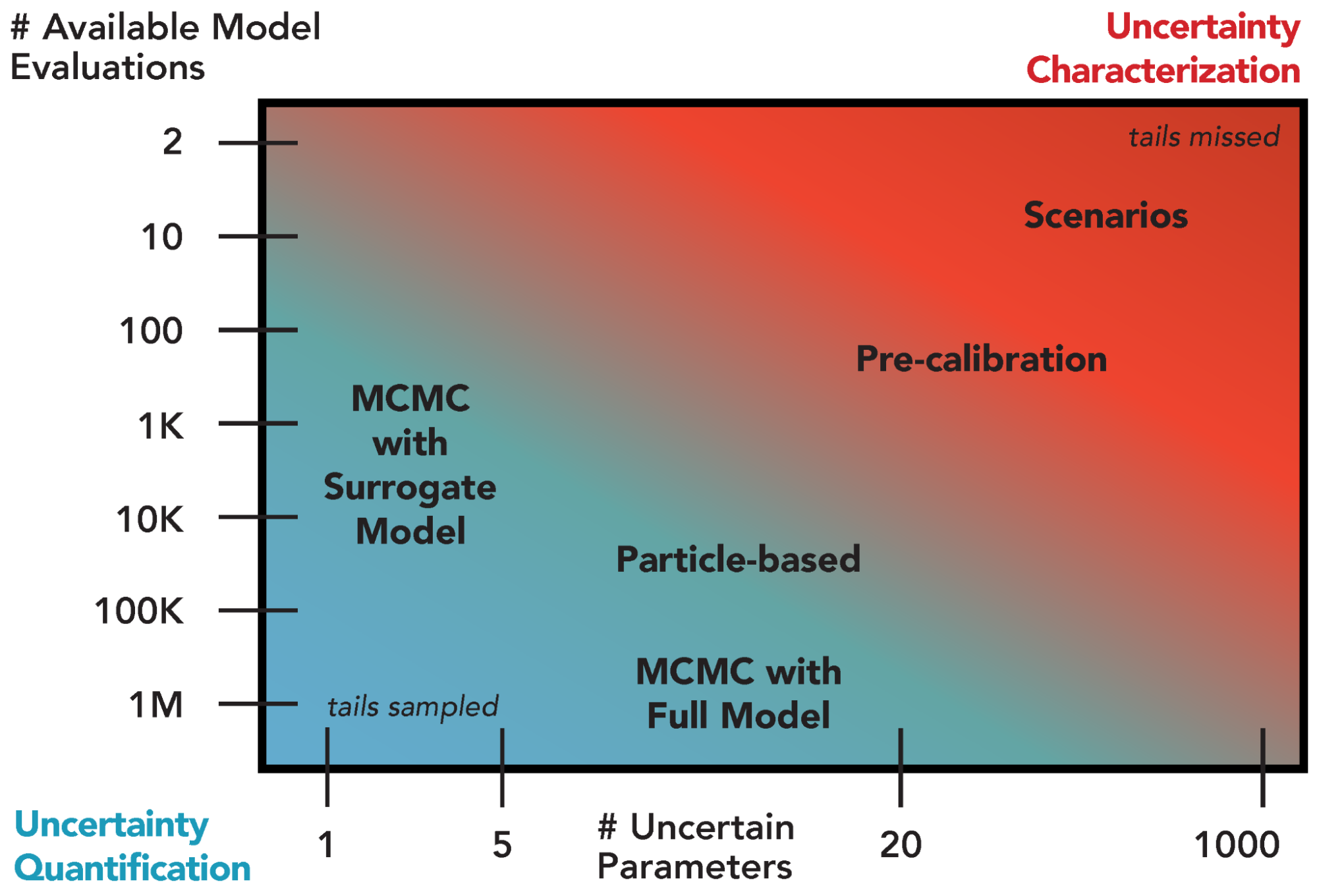
Fig. A.1 Overview of selected existing approaches for uncertainty quantification and their appropriateness given the number of uncertain model parameters and the number of available model simulations. Green shading denotes regions suitable for uncertainty quantification and red shading indicates regions more appropriate for uncertainty characterization.#
The choice of a particular UQ method depends on both the desired level of quantification and the ability to navigate the tradeoff between computational expense and the number of uncertain parameters (Fig. A.1). For example, Markov chain Monte Carlo with a full system model can provide an improved representation of uncertainty compared to the coarser pre-calibration approach [157], but requires many more model evaluations. The use of a surrogate model to approximate the full system model can reduce the number of needed model evaluations by several orders of magnitude, but the uncertainty quantification can only accommodate a limited number of parameters.
The remainder of this appendix will focus on introducing workflows for particular UQ methods, including a brief discussion of advantages and limitations.
A.2. Parametric Bootstrap#
The parametric bootstrap [158] refers to a process of model recalibration to alternate realizations of the data. The bootstrap was originally developed to estimate standard errors and confidence intervals without ascertaining key assumptions that might not hold given the available data. In a setting where observations can be viewed as independent realizations of an underlying stochastic process, a sufficiently rich dataset can be treated as a population representing the data distribution. New datasets are then generated by resampling from the data with replacement, and the model can be refit to each new dataset using maximum-likelihood estimation. The resulting distribution of estimates can then be viewed as a representation of parametric uncertainty.
A typical workflow for the parametric bootstrap is shown in Fig. A.2. After identifying outputs of interest and preparing the data, the parametric model is fit by some procedure such as minimizing root-mean-square-error or maximizing the likelihood. Alternate datasets are constructed by resampling from the population or by generating new samples from the fitted data-generating process. It is important at this step that the resampled quantities are independent of one another. For example, in the context of temporally- or spatially-correlated data, such as time series, the raw observations cannot be treated as independent realizations. However, the residuals resulting from fitting the model to the data could be (depending on their structure). For example, if the residuals are treated as independent, they can then be resampled with replacement, and these residuals added to the original model fit to create new realizations. If the residuals are assumed to be the result of an autoregressive process, this process could be fit to the original residual series and new residuals be created using this model [159]. The model is then refit to each new realization.
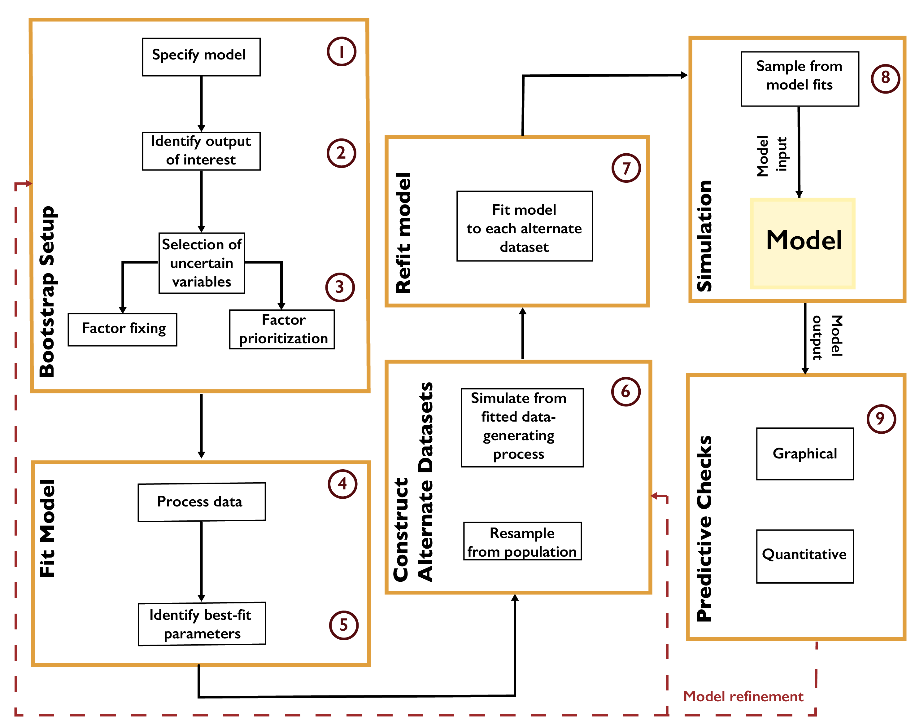
Fig. A.2 Workflow for the parametric bootstrap.#
The bootstrap is computationally convenient, particularly as the process of fitting the model to each realization can be easily parallelized. This approach also requires minimal prior assumptions. However, due to the assumption that the available data are representative of the underlying data distribution, the bootstrap can neglect key uncertainties which might influence the results. For example, when using an autoregressive process to generate new residuals, uncertainty in the autocorrelation parameter and innovation variance is neglected, which may bias estimates of, for example, low-probability but high-impact events [160].
A.3. Pre-Calibration#
Pre-calibration [18, 161, 162] involves the identification of a plausible set of parameters using some prespecified screening criterion, such as the distance from the model results to the observations (based on an appropriate metric for the desired matching features, such as root-mean-squared error). A typical workflow is shown in Fig. A.3. Parameter values are obtained by systematically sampling the input space (see Chapter 3.3). After the model is evaluated at the samples, only those passing the distance criterion are retained. This selects a subset of the parameter space as “plausible” based on the screening criterion, though there is no assignment of probabilities within this plausible region.
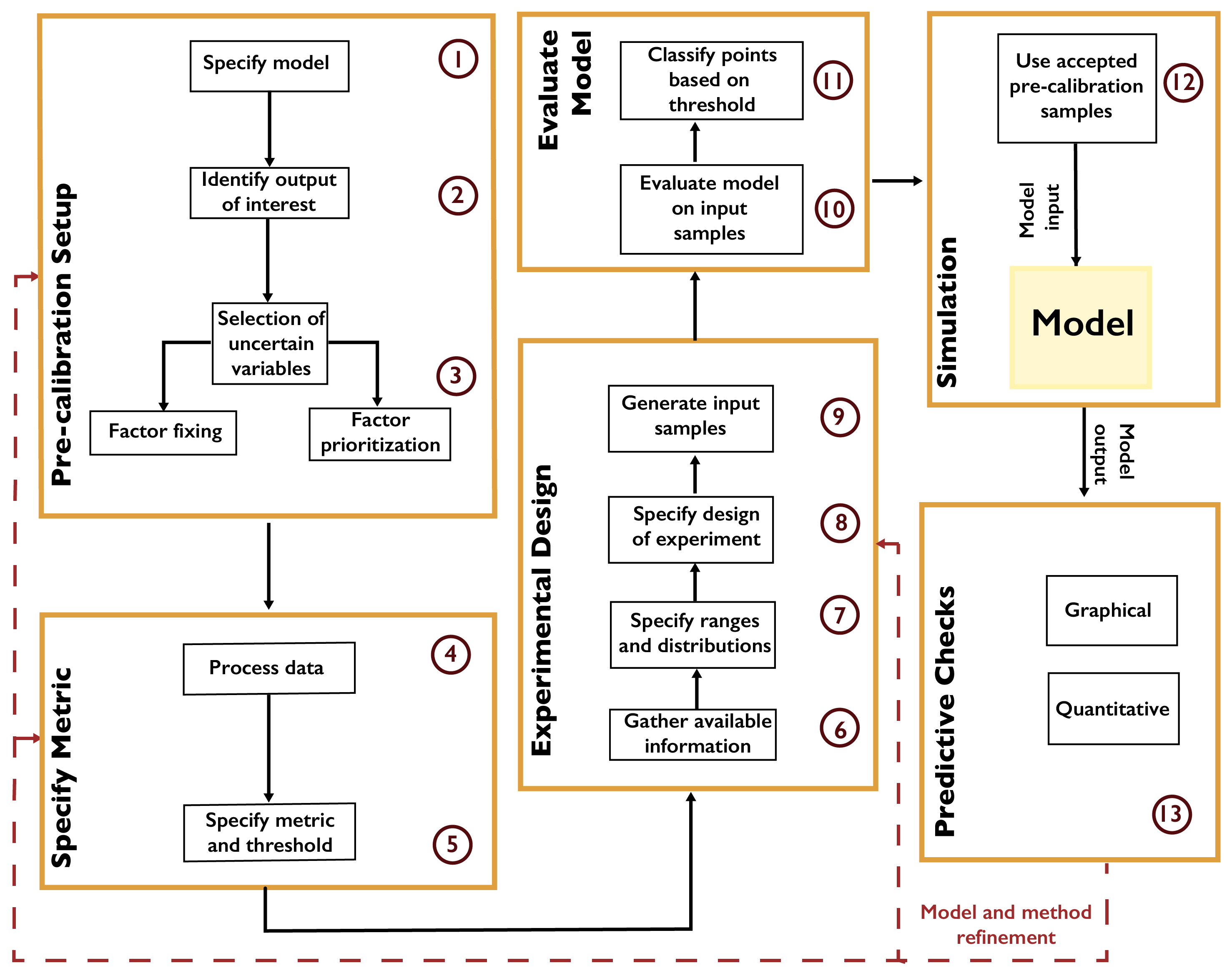
Fig. A.3 Workflow for pre-calibration.#
Pre-calibration can be useful for models which are inexpensive enough that a reasonable number of samples can be used to represent the parameter space, but which are too expensive to facilitate full uncertainty quantification. High-dimensional parameter spaces, which can be problematic for the uncertainty quantification methods below, may also be explored using pre-calibration. One key prerequisite to using this method is the ability to place a meaningful distance metric on the output space.
However, pre-calibration results in a very coarse characterization of uncertainty, especially when considering a large number of parameters, as more samples are needed to fully characterize the parameter space. Due to the inability to evaluate the relative probability of regions of the parameter space beyond the binary plausible-and-implausible characterization, pre-calibration can also result in degraded hindcast and projection skills and parameter estimates [157, 163, 164].
A related method, widely used in hydrological studies, is generalized likelihood uncertainty estimation, or GLUE [18]. Unlike pre-calibration, the underlying argument for GLUE relies on the concept of equifinality [165], which posits that it is impossible to find a uniquely well-performing parameter vector for models of abstract environmental systems [165, 166]. In other words, there exist multiple parameter vectors which perform equally or similarly well. As with pre-calibration, GLUE uses a goodness-of-fit measure (though this is called a “likelihood” in the GLUE literature, as opposed to a statistical likelihood function [167]) to evaluate samples. After setting a threshold of acceptable performance with respect to that measure, samples are evaluated and classified into “behavioral” or “non-behavioral” according to the threshold.
A.4. Markov Chain Monte Carlo#
Markov chain Monte Carlo (MCMC) is a “gold standard” approach to full uncertainty quantification. MCMC refers to a category of algorithms which systematically sample from a target distribution (in this case, the posterior distribution) by constructing a Markov chain. A Markov chain is a probabilistic structure consisting of a state space, an initial probability distribution over the states, and a transition distribution between states. If a Markov chain satisfies certain properties [168, 169], the probability of being in each state will eventually converge to a stable, or stationary, distribution, regardless of the initial probabilities.
MCMC algorithms construct a Markov chain of samples from a parameter space (the combination of model and statistical parameters). This Markov chain is constructed so that the stationary distribution is a target distribution, in this case the (Bayesian) posterior distribution. As a result, after the transient period, the resulting samples can be viewed as a set of dependent samples from the posterior (the dependence is due to the autocorrelation between samples resulting from the Markov chain transitions). Expected values can be computed from these samples (for example, using batch-means estimators [170]), or the chain can be sub-sampled or thinned and the resulting samples used as independent Monte Carlo samples due to the reduced or eliminated autocorrelation.
A general workflow for MCMC is shown in Fig. A.4. The first decision is whether to use the full model or a surrogate model (or emulator). Typical surrogates include Gaussian process emulation [171, 172], polynomial chaos expansions [173, 174], support vector machines [175, 176], and neural networks [177, 178]. Surrogate modeling can be faster, but requires a sufficient number of model evaluations for the surrogate to accurately represent the model’s response surface, and this typically limits the number of parameters which can be included in the analysis.
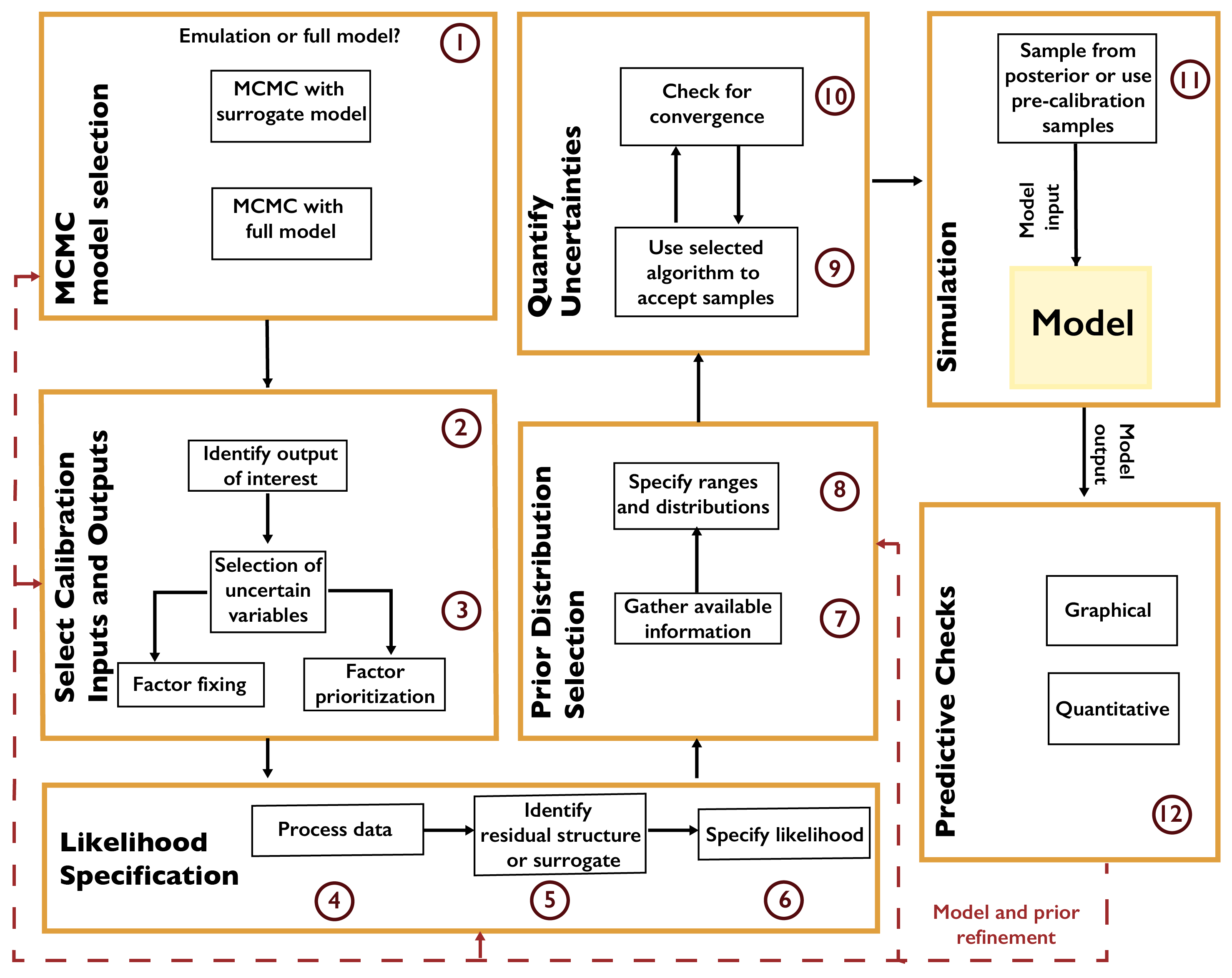
Fig. A.4 Workflow for Markov chain Monte Carlo.#
After selecting the variables which will be treated as uncertain, the next step is to specify the likelihood based on the selected surrogate model or the structure of the data-model residuals. For example, it may not always be appropriate to treat the residuals as independent and identically distributed (as is commonly done in linear regression). A mis-specification of the residual structure can result in biases and over- or under-confident inferences and projections [179].
After specifying the prior distributions (see Chapter A.6), the selected MCMC algorithm should be used to draw samples from the posterior distribution. There are many MCMC algorithms, all of which have advantages and disadvantages for a particular problem. These include the Metropolis-Hastings algorithm [169] and Hamiltonian Monte Carlo [180, 181]. Software packages typically implement one MCMC method, sometimes designed for a particular problem setting or likelihood specification. For example, R’s adaptMCMC implements an adaptive Metropolis-Hastings algorithm [182], while NIMBLE [183, 184] uses a user-customizable Metropolis-Hastings implementation, as well as functionality for Gibbs sampling (which is a special case of Metropolis-Hastings where the prior distribution has a convenient mathematical form). Some recent implementations, such as Stan [185], pyMC3 [186], and Turing [187] allow different algorithms to be used.
A main consideration when using MCMC algorithms is testing for convergence to the target distribution. As convergence is guaranteed only for a sufficiently large number of transitions, it is impossible to conclude for certain that a chain has converged for a fixed number of iterations. However, several heuristics have been developed [170, 188] to increase evidence that convergence has occurred.
A.5. Other Methods#
Other common methods for UQ exist. These include sequential Monte Carlo, otherwise known as particle filtering [189, 190, 191], where a number of particles are used to evaluate samples. An advantage of sequential Monte Carlo is that the vast majority of the computation can be parallelized, unlike with standard MCMC. A major weakness is the potential for degeneracy [190], where many particles have extremely small weights, resulting in the effective use of only a few samples.
Another method is approximate Bayesian computation (ABC) [192, 193, 194]. ABC is a likelihood-free approach that compares model output to a set of summary statistics. ABC is therefore well-suited for models and residual structures which do not lend themselves to a computationally-tractable likelihood, but the resulting inferences are known to be biased if the set of summary statistics is not sufficient, which can be difficult to know a-priori.
A.6. The Critical First Step: How to Choose a Prior Distribution#
Prior distributions play an important role in Bayesian uncertainty quantification, particularly when data is limited relative to the dimension of the model. Bayesian updating can be thought of as an information filter, where each additional datum is added to the information contained in the prior; eventually, the prior makes relatively little impact. In real world problems, it can be extremely difficult to assess how much data is required for the choice of prior to become less relevant. The choice of prior can also be influential when conducting SA prior to or without UQ. This is because a prior distribution for a sensitivity analysis for a given parameter which is much wider than the region where the model response surface is sensitive to the parameter value might cause the sensitivity calculation to underestimate the response in that potentially critical region. Similarly, a prior which is too narrow may miss regions where the model responds to the parameter altogether.
Ideally, prior distributions are constructed independently of any analysis of the new data considered. This is because using data to inform the prior as well as to compute the likelihood reuses information in a potentially inappropriate way, which can lead to overconfident inferences. Following Jaynes [195], Gelman et al. [196] refers to the ideal prior as one which encodes all available information about the model. For practical reasons (difficulty of construction or computational inconvenience), most priors fail to achieve this ideal. These compromises mean that priors should be transparently articulated and justified, so that the impact of the choice of prior can be fully understood. When there is ambiguity about an appropriate prior, such as how fat the tails should be, an analyst should examine how sensitive the UQ results are to the choice of prior.
Priors can also be classified in terms of the information encoded by them, demonstrated in Fig. A.5. Non-informative priors (illustrated in Fig. A.5 (a)) allegedly correspond to (and are frequently justified by) a position of ignorance. A classic example is the use of a uniform distribution. A uniform prior can, however, be problematic, as it can lead to improper inferences by giving extremely large values the same prior probability as values which may seem more likely [196, 197], and therefore does not really reflect a state of complete ignorance. In the extreme case of a uniform prior over the entire real line, every particular region has effectively a prior weight of zero, even though not all regions are a priori unlikely [197]. Moreover, a uniform prior which excludes possible parameter values is not actually noninformative, as it assigns zero probability to those values while jumping to a nonzero probability as soon as the boundary is crossed. While a uniform prior can be problematic for the task of uncertainty quantification, it may be useful for an initial sensitivity analysis to identify the boundary of any regions where the model is sensitive to the parameter.
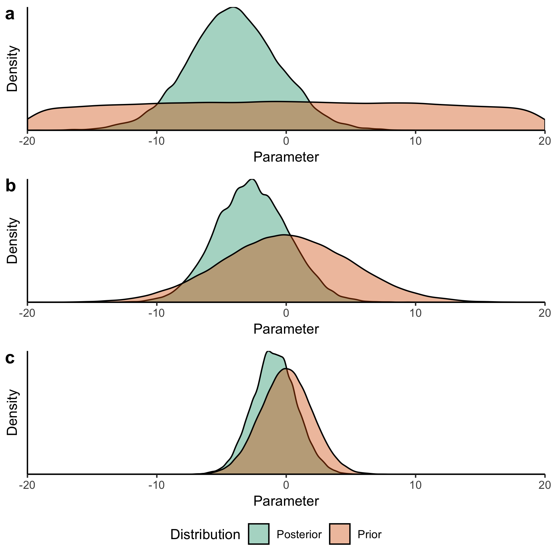
Fig. A.5 Impact of priors on posterior inferences. These plots show the results of inference for a linear regression model with 15 data points. The true value of the parameter is equal to -3. All priors have mean 0. In panel (a), a non-informative prior allows the tails of the posterior to extend freely, which may result in unreasonably large parameter values. In panel (b), a weakly informative prior constrains the tails more, but allows them to extend without too much restriction. In panel (c), an informative prior strongly constrains the tails of the posterior and biases the inference closer towards the prior mean (the posterior mean is -0.89 in this case, and closer to -3 in the other two cases).#
Informative priors strongly bound the range of probable values (illustrated in Fig. A.5 (c)). One example is a Gaussian distribution with a relatively small standard deviation, so that large values are assigned a close to null prior probability. Another example is the jump from zero to non-zero probability occurring at the truncation point of a truncated Gaussian, which could be justified based on information that the parameter cannot take on values beyond this point. Without this type of justification, however, priors may be too informative, failing to allow the information contained in the available data to update them.
Finally, weakly informative priors (illustrated in Fig. A.5 (b)) fall in between [196]. They regularize better than non-informative priors, but allow for more inference flexibility than fully informative priors. An example might be a Gaussian distribution with a moderate standard deviation, which still assigns negligible probability for values far away from the mean, but is less constrained than a narrow Gaussian for a reasonably large area. A key note is that it is not necessarily better to be more informative if this cannot be justified by the available information.
A.7. The Critical Final Step: Predictive Checks#
Every UQ workflow requires a number of choices, potentially including selecting prior distributions, the likelihood specification, and any used numerical models. Checking the appropriateness of these choices is an essential step for sound inferences, as misspecification can produce biased results [179]. Model checking in this fashion is part of an iterative UQ process, as the results can reveal adjustments to the statistical model or the need to select a different numerical model [198, 199, 200].
A classic example is the need to check the structure of residuals for correlations. Many standard statistical models, such as linear regression, assume that the residuals are independent and identically distributed from the error distribution. The presence of correlations, including temporal autocorrelations and spatial correlations, indicates a structural mismatch between the likelihood and the data. In these cases, the likelihood should be adjusted to account for these correlations.
Checking residuals in this fashion is one example of a predictive check (or a posterior predictive check in the Bayesian setting). One way to view UQ is as a means to recover data-generating processes (associated with each parameter vector) consistent with the observations. Predictive checks compare the inferred data-generating process to the observations to determine whether the model is capable of appropriately capturing uncertainty. After conducting the UQ analysis, alternatively realized datasets are simulated from sampled parameters. These alternative datasets, or their summary statistics, can be tested against the observations to determine adequacy of the fit. Predictive checks are therefore a way of probing various model components to identify shortcomings that might result in biased inferences or poor projections, depending on the goal of the analysis.
One example of a graphical predictive check for time series models is hindcasting, where predictive intervals are constructed from the alternative datasets and plotted along with the data. Hindcasts demonstrate how well the model is capable of capturing the broader dynamics of the data, as well as whether the parameter distributions produce appropriate levels of output uncertainty. A related quantitative check is the surprise index, which calculates the percentage of data points located within a fixed predictive interval. For example, the 90% predictive interval should contain approximately 90% of the data. More uncertainty than this reflects underconfidence, while less uncertainty reflects overconfidence. This could be the result of priors that are not appropriately informative, or a likelihood that does not account for correlations between data points appropriately. It could also be the result of a numerical model that isn’t sufficiently sensitive to the parameters that are treated as uncertain.
A.8. Key Take-Home Points#
When appropriate, UQ is an important component of the exploratory modeling workflow. While a number of parameter sets could be consistent with observations, they may result in divergent model outputs when exposed to different future conditions. This can result in identifying risks which are not visible when selecting a “best fit” parameterization. Quantifying uncertainties also allows us to quantify the support for hypotheses, which is an essential part of the scientific process.
Due to the scale and complexity of the experiments taking place in IM3, UQ has not been extensively used. The tradeoff between the available number of function evaluations and the number of uncertain parameters illustrated in Fig. A.1 is particularly challenging due to the increasing complexity of state-of-the-art models and the movement towards coupled, multisector models. This tradeoff can be addressed somewhat through the use of emulators and parallelizable methods. In particular, when attempting to navigate this tradeoff by limiting the number of uncertain parameters, it is important to carefully iterate with sensitivity analyses to ensure that critical parameters are identified.
Specifying prior distributions and likelihoods is an ongoing challenge. Prior distributions, in particular, should be treated as deeply uncertain when appropriate. One key advantage of the methods described in this chapter is that they have the potential for increased transparency. When it is not possible to conduct a sensitivity analysis on a number of critical priors due to limited computational budgets, fully specifying and providing a justification for the utilized distributions allows other researchers to identify key assumptions and build on existing work. The same is true for the specification of likelihoods—while likelihood-free methods avoid the need to specify a likelihood function, they require other assumptions or choices, which should be described and justified as transparently as possible.
We conclude this appendix with some key recommendations: 1. UQ analysis does not require full confidence in priors and likelihoods. Rather, UQ should be treated as part of an exploratory modeling workflow, where hypotheses related to model structures, prior distributions, and likelihoods can be tested. 2. For complex multisectoral models, UQ will typically require the use of a reduced set of parameters, either through emulation or by fixing the others to their best-fit values. These parameters should be selected through a careful sensitivity analysis. 3. Avoid the use of supposedly “non-informative” priors, such as uniform priors, whenever possible. In the absence of strong information about parameter values, the use of weakly informative priors, such as diffuse normals, is preferable. 4. Be cognizant of the limitations of conclusions that can be drawn by using each method. The bootstrap, for example, may result in overconfidence if the dataset is limited and is not truly representative of the underlying stochastic process. 5. When using MCMC, Markov chains can not be shown to have converged to the target distribution, but rather evidence can be collected to demonstrate that it is likely that they have. 6. Conduct predictive checks based on the assumptions underlying the choices made in the analysis, and iteratively update those choices if the assumptions prove to be ill-suited for the problem at hand.