4. Sensitivity Analysis: Diagnostic & Exploratory Modeling#
4.1. Understanding Errors: What Is Controlling Model Performance?#
Sensitivity analysis is a diagnostic tool when reconciling model outputs with observed data. It is helpful for clarifying how and under what conditions modeling choices (structure, parameterization, data inputs, etc.) propagate through model components and manifest in their effects on model outputs. This exploration is performed through carefully designed sampling of multiple combinations of input parameters and subsequent evaluation of the model structures that are emerging as controlling factors. Model structure and parameterization are two of the most commonly explored aspects of models that have been a central focus when evaluating their performance relative to available observations [17]. Addressing these issues plays an important role in establishing credibility in model predictions, particularly in the positivist natural sciences literature. Traditional model evaluations compare the model with observed data, and then rely on expert judgements of its acceptability based on the closeness between simulation and observation with one or a small number of selected metrics. This approach can be myopic, as it is often impossible to use one metric to attribute a certain error and to link that with different parts of the model and its parameters [127]. This means that, even when the error or fitting measure between the model estimates and observations is very small, it is not guaranteed that all the components in the model accurately represent the conceptual reality that the model is abstracting: propagated errors in different parts of the model might cancel each other out, or multiple parameterized implementations of the model can yield similar performance (i.e., equifinality [17]).
The inherent complexity of a system hinders accepting or rejecting a model based on one performance measure and different types of measures can aid in evaluating the various components of a model as essentially a multiobjective problem [25, 26]. In addition, natural systems mimicked by the models contain various interacting components that might act differently across spatial and temporal domains [51, 55]. This heterogeneity is lost when a single performance measure is used, as a highly dimensional and interactive system becomes aggregated through the averaging of spatial or temporal output errors [15]. Therefore, diagnostic error analyses should consider multiple error signatures across different scales and states of concern when seeking to understand how model performance relates to observed data (Fig. 4.1). Diverse error signatures can be used to measure the consistency of underlying processes and behaviors of the model and to evaluate the dynamics of model controls under changing temporal and spatial conditions [128]. Within this framework, even minimal information extracted from the data can be beneficial as it helps us unearth structural inadequacies in the model. In this context, proper selection of measures of model performance and the number of measures could play consequential roles in our understanding of the model and its predictions [129].
As discussed earlier, instead of the traditional focus on using deterministic prediction that results in a single error measure, many plausible states and spaces could be searched for making different inferences and quantifying uncertainties. This process also requires estimates of prior probability distributions of all the important parameters and quantification of model behavior across input space. One strategy to reduce the search space is filtering of some model alternatives that are not consistent with observations and known system behaviors. Those implausible parts of the search space can be referred to as non-physical or non-behavioral alternatives [50, 104]. This step is conducted before the Bayesian calibration exercise (see Chapter A).
A comprehensive model diagnostic workflow typically entails the components demonstrated in Fig. 4.1. The workflow begins with the selection of model input parameters and their plausible ranges. After the parameter selection, we need to specify the design of experiment (Chapter 3.3) and the sensitivity analysis method (Chapter 3.4) to be used. As previously discussed, these methods require different numbers of model simulations, and each method provides a different insights into the direct effects and interactions of the uncertain factors. In addition, the simulation time of the model and the available computational resources are two of the primary considerations that influence these decisions. After identifying the appropriate methods, we generate a matrix of input parameters, where each set of input parameters will be used to conduct a model simulation. The model can include one or more output variables that fluctuate in time and space. The next step is to analyze model performance by comparing model outputs with observations. As discussed earlier, the positivist model evaluation paradigm focuses on a single model performance metric (error), leading to a loss of information about model parameters and the suitability of the model’s structure. However, a thorough investigation of the temporal and spatial signatures of model outputs using various performance metrics or time- and space-varying sensitivity analyses can shed more light on the fitness of each parameter set and the model’s internal structure. This analysis provides diagnostic feedback on the importance and range of model parameters and can guide further improvement of the model algorithm.
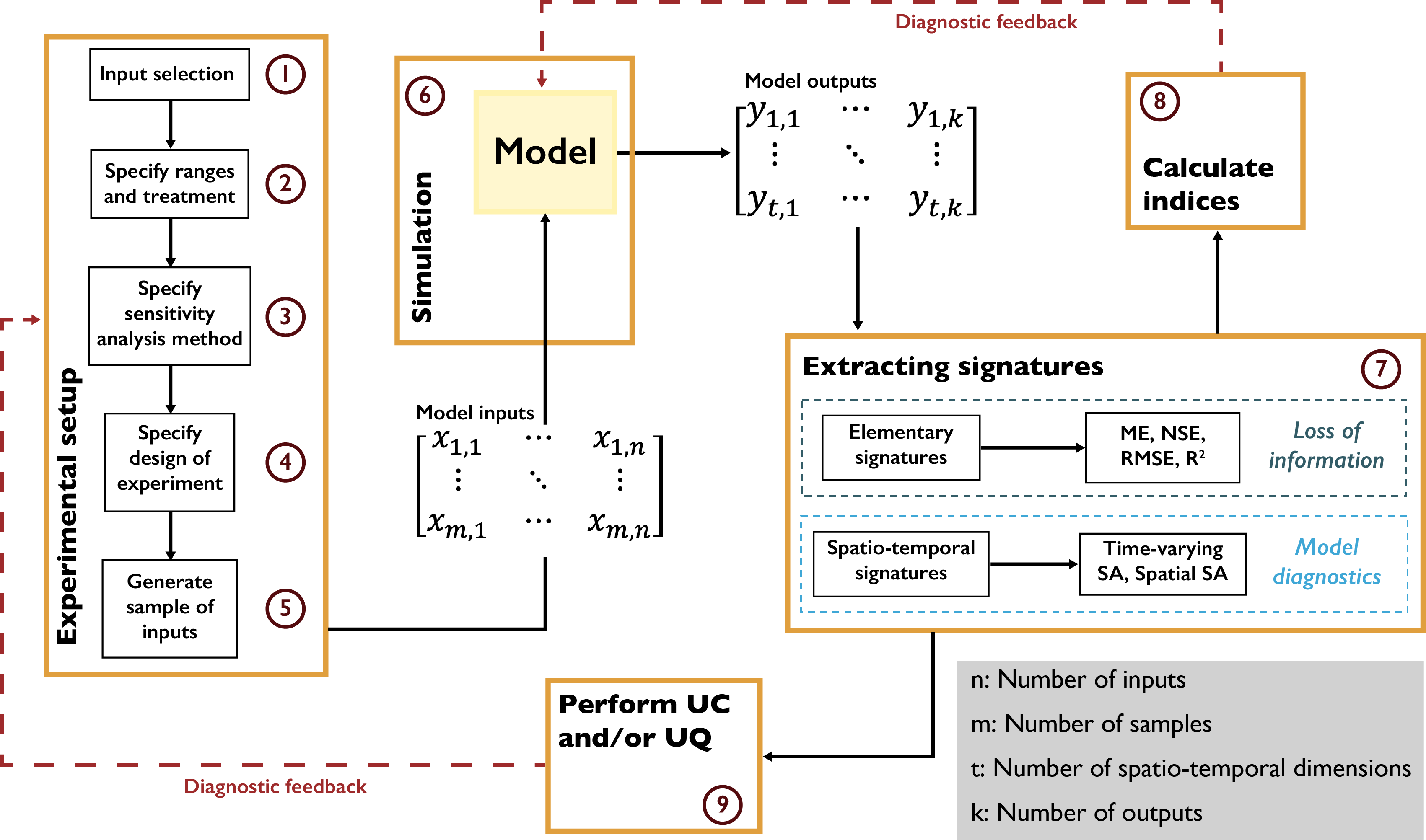
Fig. 4.1 Diagnostic evaluation of model fidelity using sensitivity analysis methods.#
Note
Put this into practice! Click the following badge to try out an interactive tutorial on implementing a time-varying sensitivity analysis of HYMOD model parameters: HYMOD Jupyter Notebook
4.2. Consequential Dynamics: What is Controlling Model Behaviors of Interest?#
Consequential changes in dynamic systems can take many forms, but most dynamic behavior can be categorized in a few basic patterns. Feedback structures inherent in a system, be they positive or negative, generate these patterns which can be grouped into three groups for the simplest of systems: exponential growth, goal seeking, and oscillation (Fig. 4.2). A positive (or self-reinforcing) feedback gives rise to exponential growth, a negative (or self-correcting) feedback gives rise to a goal seeking mode, and negative feedbacks with time delays give rise to oscillatory behavior. Nonlinear interactions between the system’s feedback structures can give rise to more complex dynamic behavior modes, examples of which are also shown in Fig. 4.2, adapted from Sterman [130].

Fig. 4.2 Common modes of behavior in dynamic systems, occurring based on the presence of positive and negative feedback relationships, and linear and non-linear interactions. Adapted from Sterman [130].#
The nature of feedback processes in a dynamic system shapes its fundamental behavior: positive feedbacks generate their own growth, negative feedbacks self-limit, seeking balance and equilibrium. In this manner, feedback processes give rise to different regimes, multiples of which could be present in each mode of behavior. Consider a population of mammals growing exponentially until it reaches the carrying capacity of its environment (referred to as S-shaped growth). When the population is exponentially growing, the regime is dominated by positive feedback relationships that reinforce its growth. As the population approaches its carrying capacity limit, negative feedback structures begin to dominate, counteracting the growth and establishing a stable equilibrium. Shifts between regimes can be thought of as tipping points, mathematically defined as unstable equilibria, where the presence of positive feedbacks amplifies disturbances and moves the system to a new equilibrium point. In the case of stable equilibria, the presence of negative feedbacks dampens any small disturbance and maintains the system at a stable state. As different feedback relationships govern each regime, different factors (those making up each feedback mechanism) are activated and shape the states the system is found in, as well as define the points of equilibria.
For simple stylized models with a small number of states, system dynamics analysis can analytically derive these equilibria, the conditions for their stability and the factors determining them. The ability for this to be performed is, however, significantly challenged when it comes to systems that attempt to more closely resemble real complex systems. We argue this is the case for several reasons. First, besides generally exhibiting complex nonlinear dynamics, real world systems are also made up from larger numbers of interacting elements, which often makes the analytic derivation of system characteristics intractable [131, 132]. Second, human-natural systems temporally evolve and transform when human state-aware action is present. Consider, for instance, humans recreationally hunting the aforementioned population of mammals. Humans act based on the mammal population levels by enforcing hunting quotas or establishing protected territories or eliminating other predators. The mammal population reacts in a response, giving birth to ever changing state-action-consequence feedbacks, the path dependencies of which become difficult to diagnose and understand (e.g., [133]). Trying to simulate the combination of these two challenges (large numbers of state-aware agents interacting with a natural resource and with each other) produces intractable models that require advanced heuristics to analyze their properties and establish useful inferences.
Sensitivity analysis paired with exploratory modeling methods offers a promising set of tools to address these challenges. We present a simple demonstrative application based on Quinn et al. [134]. This stylistic example was first developed by Carpenter et al. [135] and represents a town that must balance its agricultural and industrial productivity with the pollution it creates in a downstream lake. Increased productivity allows for increased profits, which the town aims to maximize, but it also produces more pollution for the lake. Too much phosphorus pollution can cause irreversible eutrophication, a process known as “tipping” the lake. The model of phosphorus in the lake \(X_t\) at time \(t\) is governed by:
where \(a_t \in [0,0.1]\) is the town’s pollution release at each timestep, \(b\) is the natural decay rate of phosphorus in the lake, \(q\) defines the lake’s recycling rate (primarily through sediments), and \(\varepsilon\) represents uncontrollable natural inflows of pollution modeled as a log-normal distribution with a given mean, \(\mu\), and standard deviation \(\sigma\).
Panels (a-c) in Fig. 4.3 plot the fluxes of phosphorus into the lake versus the mass accumulation of phosphorus in the lake. The red line corresponds to the phosphorus sinks in the lake (natural decay), given by \(bX_t\). The grey shaded area represents the lake’s phosphorus recycling flux, given by \(\frac{X_{t}^q} {1+X_{t}^q}\). The points of intersection indicate the system’s equilibria, two of which are stable, and one is unstable (also known as the tipping point). The stable equilibrium in the bottom left of the figure reflects an oligotrophic lake, whereas the stable equilibrium in the top right represents a eutrophic lake. With increasing phosphorus values, the tipping point can be crossed, and the lake will experience irreversible eutrophication, as the recycling rate would exceed the removal rate even if the town’s pollution became zero. In the absence of anthropogenic and natural inflows of pollution in the lake (\(a_t\) and \(\varepsilon\) respectively), the area between the bottom-left black point and the white point in the middle can be considered as the safe operating space, before emission levels cross the tipping point.
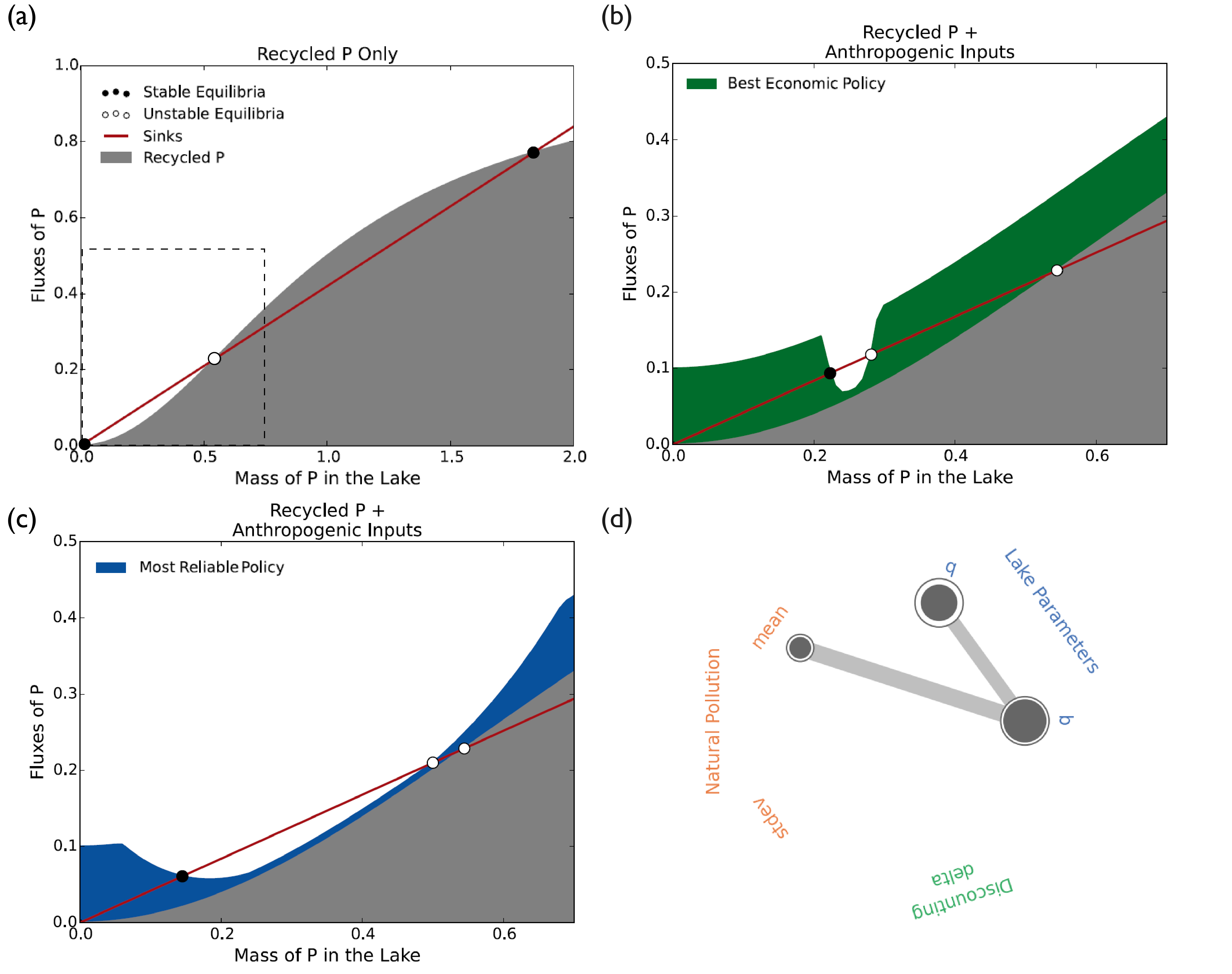
Fig. 4.3 Fluxes of phosphorus with regards to mass of phosphorus in the lake and sensitivity analysis results, assuming \(b=0.42\) and \(q=2\). (a) Fluxes of phosphorus assuming no emmisions policy and no natural inflows. (b-c) Fluxes phosphorus when applying two different emissions policies. The “Best economic policy” and the “Most reliable policy” have been identified by Quinn et al. [134] and can be found at Quinn [136]. (d) Results of a sensitivity analysis on the parameters of the model most consequential to the reliability of the “Most reliable policy”. The code to replicate the sensitivity analysis can be found at Hadka [137]. Panels (a-c) are used courtesy of Julianne Quinn, University of Virginia.#
The town has identified two potential policies that can be used to manage this lake, one that maximizes its economic profits (“best economic policy”) and one that maximizes the time below the tipping point (“most reliable policy”). Panels (b-c) in Fig. 4.3 add the emissions from these policies to the recycling flux and show how the equilibria points shift as a result. In both cases the stable oligotrophic equilibrium increases and the tipping point decreases, narrowing the safe operating space [131, 138]. The best economic policy results in a much narrower space of action, with the tipping point very close to the oligotrophic equilibrium. The performance of both policies depends significantly on the system parameters. For example, a higher value of \(b\), the natural decay rate, would shift the red line upward, moving the equilibria points and widening the safe operating space. Inversely, a higher value of \(q\), the lake’s recycling rate, would shift the recycling line upward, moving the tipping point lower and decreasing the safe operating space. The assumptions under which these policies were identified are therefore critical to their performance and any potential uncertainty in the parameter values could be detrimental to the system’s objectives being met.
Sensitivity analysis can be used to clarify the role these parameters play on policy performance. Fig. 4.3 (d) shows the results of a Sobol sensitivity analysis on the reliability of the “most reliable” policy in a radial convergence diagram. The significance of each parameter is indicated by the size of circles corresponding to it. The size of the interior dark circle indicates the parameter’s first-order effects and the size of the exterior circle indicates the parameter’s total-order effects. The thickness of the lines between two parameters indicated the extent of their interaction (second-order effects). In this case, parameters \(b\) and \(q\) appear to have the most significant importance on the system, followed by the mean, \(\mu\), of the natural inflows. All these parameters function in a manner that shifts the location of the three equilibria and therefore policies that are identified ignoring this parametric uncertainty might fail to meet their intended goals.
It is worth mentioning that current sensitivity analysis methods are somewhat challenged in addressing several system dynamics analysis questions. The fundamental reason is that sensitivity analysis methods and tools have been developed to gauge numerical sensitivity of model output to changes in factor values. This is natural, as most simulation studies (e.g., all aforementioned examples) have been traditionally concerned with this type of sensitivity. In system dynamics modeling, however, a more important and pertinent concern is changes between regimes or between behavior modes (also known as bifurcations) as a result of changes in model factors [130, 139]. This poses two new challenges. First, identifying a change in regime depends on several characteristics besides a change in output value, like the rate and direction of change. Second, behavior mode changes are qualitative and discontinuous, as equilibria change in stability but also move in and out of existence.
Despite these challenges, recent advanced sensitivity analysis methods can help illuminate which factors in a system are most important in shaping boundary conditions (tipping points) between different regimes and determining changes in behavior modes. Reviewing such methods is outside the scope of this text, but the reader is directed to the examples of Eker et al. [22] and Hadjimichael et al. [133], who apply parameterised perturbation on the functional relationships of a system to study the effects of model structural uncertainty on model outputs and bifurcations, and Hekimoğlu and Barlas [139] and Steinmann et al. [140] who, following wide sampling of uncertain inputs, cluster the resulting time series in modes of behavior and identify most important factors for each.
Note
Put this into practice! Click the following badge to try out an interactive tutorial on performing a sensitivity analysis to discover consequential dynamics: Factor Discovery Jupyter Notebook
4.3. Consequential Scenarios: What is Controlling Consequential Outcomes?#
As overviewed in Chapter 2.2, most models are abstractions of systems in the real world. When sufficient confidence has been established in a model, it can then act as a surrogate for the actual system, in that the consequences of potential stressors, proposed actions or other changes can be evaluated by computer model simulations [36]. A model simulation then represents a computational experiment, which can be used to assess how the modeled system would behave should the various changes come to be. Steven Bankes coined the term exploratory modeling to describe the use of large sets of such computational experiments to investigate their implications on the system. Fig. 4.4 presents a typical workflow of an exploratory modeling application. Exploratory modeling approaches typically use sampling designs to generate large ensembles of states that represent combinations of changes happening together, spanning the entire range of potential values a factor might take (indicated in Fig. 4.4 by numbers 2-5). This perspective on modeling is particularly relevant to studies making long term projections into the future.
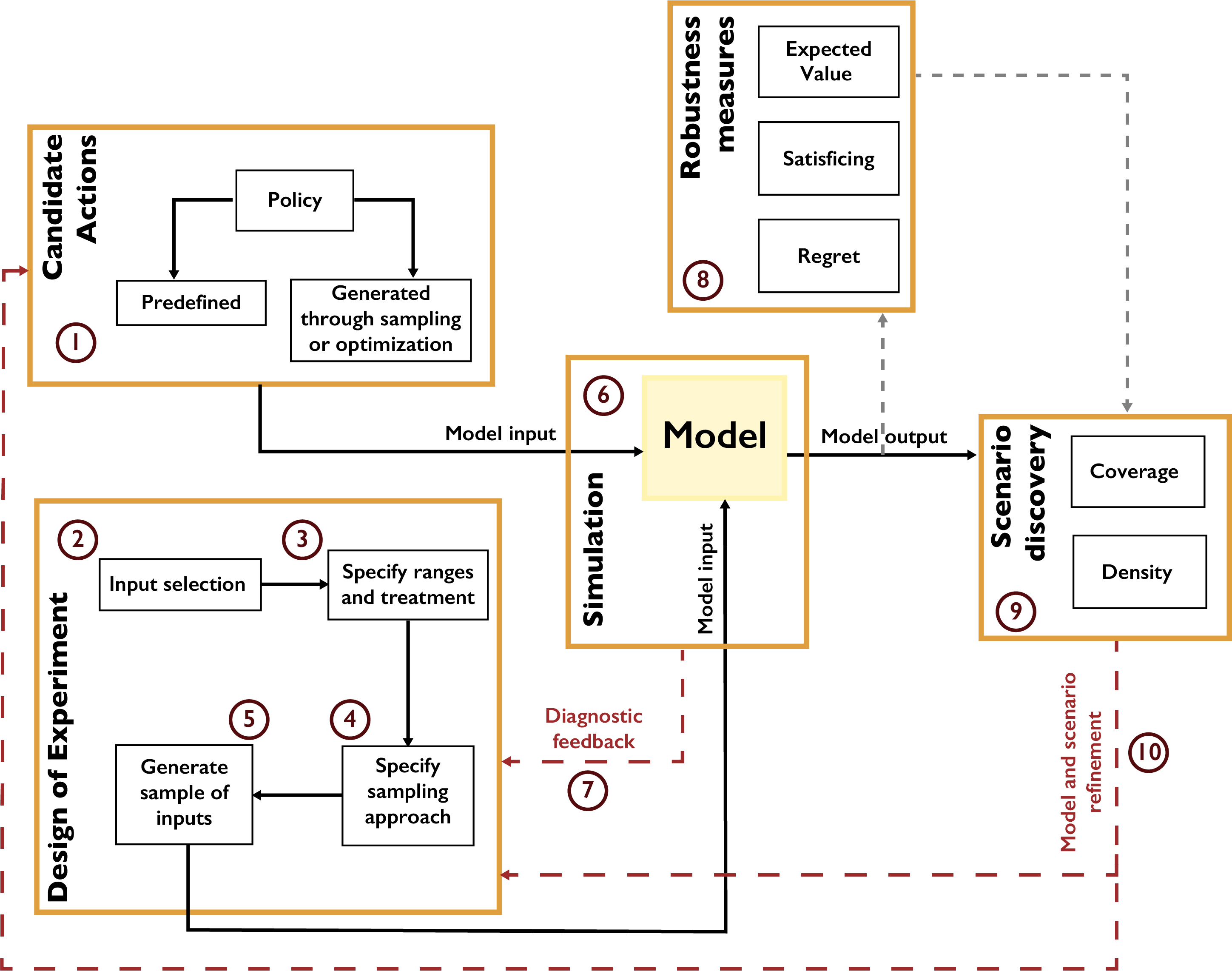
Fig. 4.4 A typical exploratory modeling workflow#
In the long-term policy analysis literature, exploratory modeling has prominently placed itself as an alternative to traditional narrative scenario or assumptions-based planning approaches, in what can be summarized in the following two-pronged critique [36, 141, 142]. The most prevalent criticism sees that the future and how it might evolve is both highly complex and deeply uncertain. Despite its benefits for interpretation and intuitive appeal, a small number of scenarios invariably misses many other potential futures that did not get selected as sufficiently representative of the future. This is especially the case for aggregate, narrative scenarios that describe simultaneous changes in multiple sectors together (e.g., “increased energy demand, combined with high agricultural land use and large economic growth”), such as the emission scenarios produced by the Intergovernmental Panel on Climate Change [143]. The bias introduced by this reduced set of potential changes can skew inferences drawn from the model, particularly when the original narrative scenarios are focused on a single or narrow set of measures of system behavior.
The second main criticism of traditional narrative scenario-based planning methods is that they provide no systematic way to distinguish which of the constituent factors lead to the undesirable consequences produced by a scenario. Narrative scenarios (e.g., the scenario matrix framework of RCPs-SSPs-SPAs; [144]) encompass multiple changes happening together selected to span the range of potential changes but are not typically generated in a systematic factorial manner that considers the multiple ways the factors can be combined. This has two critical limitations. It obfuscates the role each component factor plays in the system, both in isolation and in combination with others (e.g., “is it the increased energy demand or the high agricultural land use that cause unbearable water stress?”). It also renders the delineation of how much change in a factor is critical near impossible. Consider, for example, narrative scenario A with a 5% increase in energy demand, and scenario B with a 30% increase in energy demand, which would have dire consequences. At which point between 5% and 30% do the dire consequences actually begin to occur? Such questions cannot be answered without a wide exploration of the space of potential changes. It should be noted that for some levels of model complexity and computational demands (e.g., global-scale models) there is little feasible recourse beyond the use of narrative scenarios.
Exploratory modeling is typically paired with scenario discovery methods (indicated by number 9 in Fig. 4.4) that identify which of the scenarios (also known as states of the world) generated indeed have consequences of interest for stakeholders and policy makers, in an approach referred to as ensemble-based scenario-discovery [45, 102, 103]. This approach therefore flips the planning analysis from one that attempts to predict future system conditions to one that attempts to discover the (un)desirable future conditions. Ensemble-based scenario discovery can thus inform what modeling choices yield the most consequential behavioral changes or outcomes, especially when considering deeply uncertain, scenario-informed projections [9, 145]. The relative likelihoods and relevance of the discovered scenarios can be subsequently evaluated by the practitioners a posteriori, within a richer context of knowing the wider set of potential consequences [146]. This can include changing how an analysis is framed (number 10 in Fig. 4.4). For instance, one could initially focus on ensemble modeling of vulnerability using a single uncertain factor that is assumed to be well characterized by historical observations (e.g., streamflow; this step is represented by numbers 2-3 in Fig. 4.4). The analysis can then shift to include projections of more factors treated as deeply uncertain (e.g., urbanization, population demands, temperature, and snow-melt) to yield a far wider space of challenging projected futures. UC experiments contrasting these two framings can be highly valuable for tracing how vulnerability inferences change as the modeled space of futures expands from the historical baseline [134].
An important nuance to be clarified here is that the focus or purpose of a modeling exercise plays a major role in whether a given factor of interest is considered well-characterized or deeply uncertain. Take the example context of characterizing temperature or streamflow extremes, where for each state variable of interest for a given location of focus there is a century of historical observations. Clearly, the observation technologies will have evolved over time uniquely for temperature and streamflow measurements and they likely lack replicate experiments (data uncertainty). A century of record will be insufficient to capture very high impact and rare extreme events (i.e., increasingly poor structural/parametric inference for the distributions of specific extreme single or compound events). The mechanistic processes as well as their evolving variability will be interdependent but uniquely different for each of these state variables. A large body of statistical literature exists focusing on the topics of synthetic weather [81, 82] or streamflow [83, 84] generation that provides a rich suite of approaches for developing history-informed, well-characterized stochastic process models to better estimate rare individual or compound extremes. These history-focused approaches can be viewed as providing well-characterized quantifications of streamflow or temperature distributions; however, they do not capture how coupled natural-human processes can fundamentally change their dynamics when transitioning to projections of longer-term futures (e.g., streamflow and temperature in 2055). Consequently, changing the focus of the modeling to making long term projections of future streamflow or temperature now makes these processes deeply uncertain.
Scenario discovery methods (number 9 in Fig. 4.4) can be qualitative or quantitative and they generally attempt to distinguish futures in which a system or proposed policies to manage the system meet or miss their goals [103]. The emphasis placed by exploratory modeling on model outputs that have decision relevant consequences represents a shift toward a broader class of metrics that are reflective of the stakeholders’ concerns, agency and preferences (also discussed in Chapter 2.2). As a result, sensitivity analysis and scenario discovery methods in this context are therefore applied to performance metrics that go beyond model error but are rather focused on broader metrics such as the resilience of a sector, the reliability of a process, or the vulnerability of a population in the face of uncertainty. In exploratory modeling literature, this metric is most typically—but not always—a measure of robustness (number 8 in Fig. 13). Robustness is a property of a system or a design choice capturing its insensitivity to uncertainty and can be measured via a variety of means, most recently reviewed by Herman et al. [147] and McPhail et al. [129].
Scenario discovery is typically performed through the use of algorithms applied on large databases of model runs, generated through exploratory modeling, with each model run representing the performance of the system in one potential state of the world. The algorithms seek to identify the combinations of factor values (e.g., future conditions) that best distinguish the cases in which the system does or does not meet its objectives. The most widely known classification algorithms are the Patient Rule Induction Method (PRIM; [97]) and Classification and Regression Trees (CART; [98]). These factor mapping algorithms create orthogonal boundaries (multi-dimensional hypercubes) between states of the world that are successful or unsuccessful in meeting the system’s goals [65]. The algorithms attempt to strike a balance between simplicity of classification (and as a result, interpretability) and accuracy [45, 103, 148].
Even though these approaches have been shown to yield interpretable and relevant scenarios [149], several authors have pointed out the limitations of these methods with regards to their division of space in orthogonal behavioral and non-behavioral regions [150]. Due to their reliance on boundaries orthogonal to the uncertainty axes, PRIM and CART cannot capture interactions between the various uncertain factors considered, which can often be significant [151]. More advanced methods have been proposed to address this drawback, with logistic regression being perhaps the most prominent [151, 152, 153]. Logistic regression can produce boundaries that are not necessarily orthogonal to each uncertainty axis, nor necessarily linear, if interactive terms between two parameters are used to build the regression model. It also describes the probability that a state of the world belongs to the scenarios that lead to failure. This feature allows users to define regions of success based on a gradient of estimated probability of success in those worlds, unlike PRIM which only classifies states of the world in two regions [151, 154].
Another more advanced factor mapping method is boosted trees [99, 155]. Boosted trees can avoid two limitations inherent to the application of logistic regression: i) to build a nonlinear classification model the interactive term between two uncertainties needs to be pre-specified and cannot be discovered (e.g., we need to know a-priori whether factor \(x_1\) interacts with \(x_2\) in a relationship that looks like \(x_1\)·\(x_2\) or \(x_1^{x_2}\)); and ii) the subspaces defined are always convex. The application of such a factor mapping algorithm is limited in the presence of threshold-based rules with discrete actions in a modeled system (e.g., “if network capacity is low, build new infrastructure”), which results in failure regions that are nonlinear and non-convex [150]. Boosting works by creating an ensemble of classifiers and forcing some of them to focus on the hard-to-learn parts of the problem, and others to focus on the easy-to-learn parts. Boosting applied to CART trees can avoid the aforementioned challenges faced by other scenario discovery methods, while resisting overfitting [156], assuring the identified success and failure regions are still easy to interpret.
Below we provide an example application of two scenario discovery methods, PRIM and logistic regression, using the lake problem introduced in the previous section. From the sensitivity analysis results presented in Fig. 4.3 (d), we can already infer that parameters \(b\) and \(q\) have important effects on model outputs (i.e., we have performed factor prioritization). Scenario discovery (i.e., factor mapping) complements this analysis by further identifying the specific values of b and q that can lead to consequential and undesirable outcomes. For the purposes of demonstration, we can assume the undesirable outcome in this case is defined as the management policy failing to achieve 90% reliability in a state of the world.
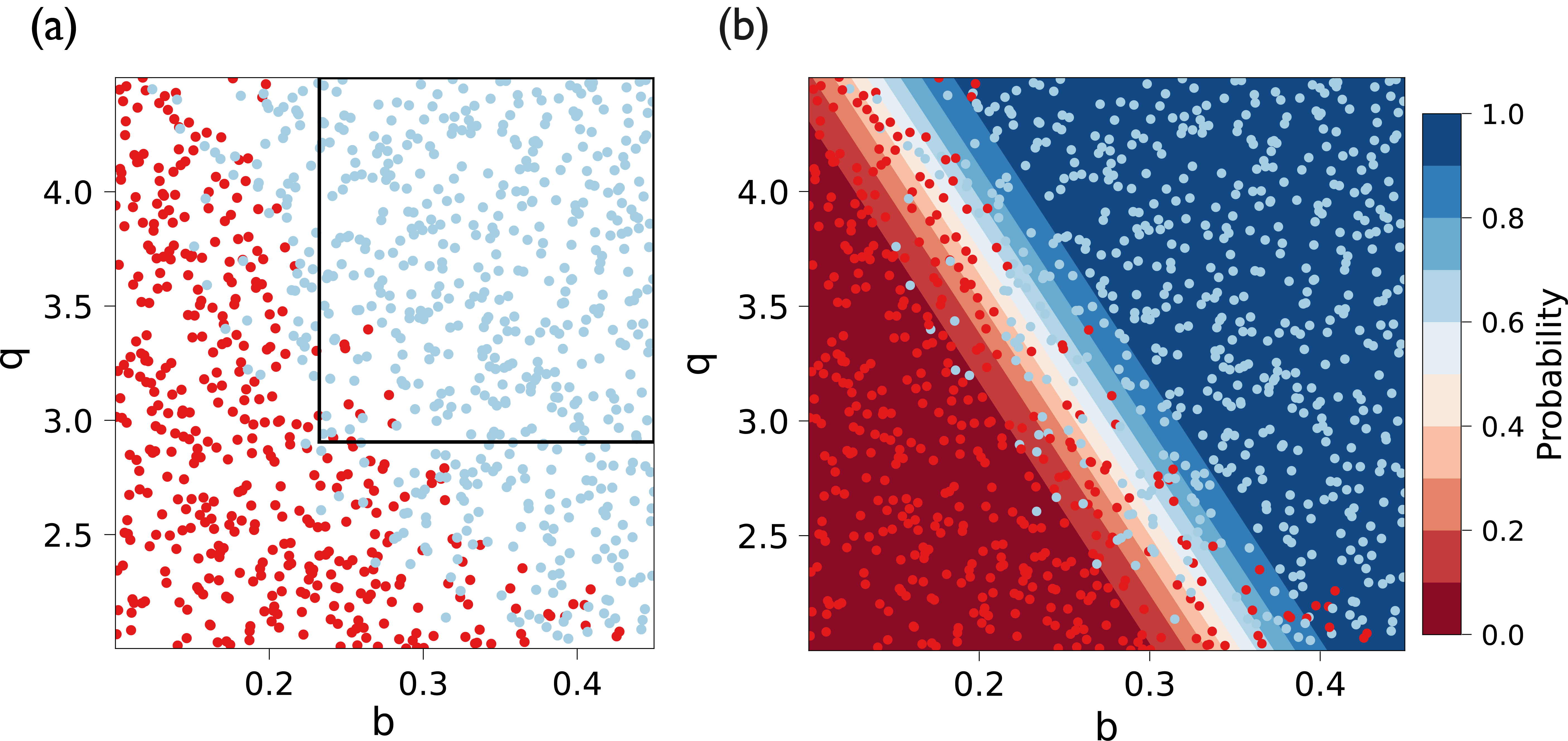
Fig. 4.5 Scenario discovery for the lake problem, using (a) PRIM and (b) logistic regression.#
Fig. 4.5 shows the results of scenario discovery, performed through (a) PRIM and (b) logistic regression. Each point in the two panels indicates a potential state of the world, generated through Latin Hypercube Sampling. Each point is colored by whether the policy meets the above performance criterion, with blue indicating success and red indicating failure. PRIM identifies several orthogonal areas of interest, one of which is shown in panel (a). As discussed above, this necessary orthogonality limits how PRIM identifies areas of success (the area within the box). As factors \(b\) and \(q\) interact in this system, the transition boundary between the regions of success and failure is not orthogonal to any of the axes. As a result, a large number of points in the bottom right and the top left of the figure are left outside of the identified region. Logistic regression can overcome this limitation by identifying a diagonal boundary between the two regions, seen in panel (b). This method also produces a gradient of estimated probability of success across these regions.
Note
Put this into practice! Click the following link to try out an interactive tutorial on performing factor mapping using logistic regression: Logistic Regression Jupyter Notebook
Note
The following articles are suggested as fundamental reading for the information presented in this section:
Gupta, H.V., Wagener, T., Liu, Y., 2008. Reconciling theory with observations: elements of a diagnostic approach to model evaluation. Hydrological Processes: An International Journal 22, 3802–3813.
Bankes, S., 1993. Exploratory Modeling for Policy Analysis. Operations Research 41, 435–449. https://doi.org/10.1287/opre.41.3.435
Groves, D.G., Lempert, R.J., 2007. A new analytic method for finding policy-relevant scenarios. Global Environmental Change 17, 73–85. https://doi.org/10.1016/j.gloenvcha.2006.11.006
The following articles can be used as supplemental reading:
Marchau, V.A.W.J., Walker, W.E., Bloemen, P.J.T.M., Popper, S.W. (Eds.), 2019. Decision Making under Deep Uncertainty: From Theory to Practice. Springer International Publishing. https://doi.org/10.1007/978-3-030-05252-2
Sterman, J.D., 1994. Learning in and about complex systems. System Dynamics Review 10, 291–330. https://doi.org/10.1002/sdr.4260100214